
14 Google Sheets Formulas Every SEO Needs To Know
Google Sheets is a powerful (and free) cloud-based tool that allows us to organize data effectively and efficiently. The secret to taking full advantage of everything Google Sheets has to offer is tapping into its extensive list of formulas.
Without a set of proficient formulas at the ready, you could spend hours sorting, splitting, merging, adding, deleting, and searching for data. On the other hand, if you know exactly which formulas to use for specific tasks, you will save yourself so much time (and, let’s be honest, mental energy).
You can also make your shareable sheets much cleaner and more manageable for yourself and anyone else who needs to use them.
What SEOs Need
As SEOs, we don’t want to spend all our time cleaning up messy spreadsheets. We want our spreadsheets to be helpful resources that work for us – simplifying tasks and presenting vital data clearly. Today, I want to share a list of basic formulas I know will help you work faster and smarter, so you have more time to spend on other tasks you love.
Maybe you are a rookie when it comes to Google Sheets, and you have no idea where to start. Or maybe you already love using this resource and want to take full advantage of everything it has to offer. Either way, the following list of formulas is a great set of tools to have on hand.
A Few Google Sheet Basics Before We Start
Before we dive into the formulas themselves, we want to cover a few fundamentals for beginners out there. Knowing these basic definitions will make it much easier to pick up on how to use the formulas we share today and others you learn in the future.
-
A cell is a single data point within a sheet.
-
A row is a set of cells that extend horizontally.
-
A column is a set of cells that extend vertically.
-
A function is an operation used to generate a desired result.
-
A formula is a combination of cells, columns, rows, functions, and ranges used to create an equation.
-
A range is the selection of cells across a column or row (or both).
-
All formulas must start with an equals sign (=).
1. VLOOKUP for Importing Data
Most SEOs agree that the VLOOKUP (V for vertical) function is one of the best tools to have in your toolbox. With it, you can pull data from one spreadsheet into another spreadsheet – as long as the two sheets share a common value.
This comes in handy when you have large sets of data you want to combine without having to go in and copy and paste the data in every single cell manually. It is especially helpful when you are working with many spreadsheets.
Let’s say I have one spreadsheet with two tabs (see screenshot below). One tab shows a list of keywords and each keyword’s monthly search volume. The second tab has the same list of keywords with their SEO difficulty scores. My goal is to pull the SEO difficulty scores into the first tab using the VLOOKUP formula:
=VLOOKUP(search_key, range, index, is_sorted)
It is important to note that the data point (in this case, “Keyword”) that I want to pull from one tab into the other must be the same in both sheets. This data point must also be located in the first column of the second tab – column A.

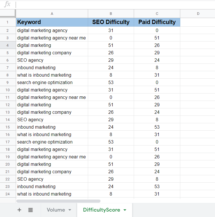
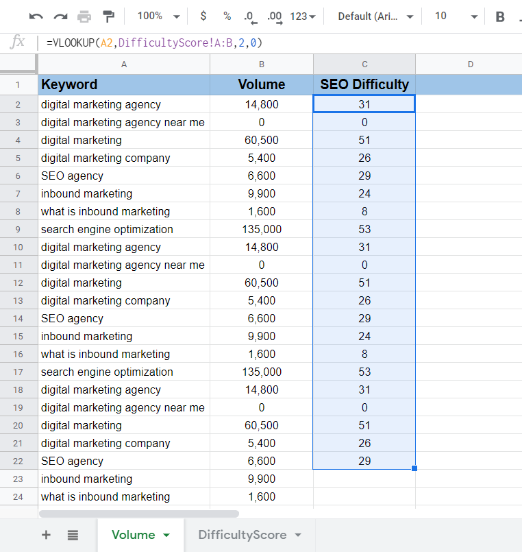
I want to pull the data from column two (DifficultyScore) into my “Volume” spreadsheet (first tab). So, here is what my formula looks like:
=VLOOKUP(A2,DifficultyScore!A:B,2,0)
Let’s break down each part of this equation:
-
Search_key is the value both sheets have in common. We will start with the first keyword in the list, located in cell A2.
-
Range is where you insert the name of the tab you are pulling data from, along with the range of columns you want your formula to read. I want to pull in columns A (Keyword) and B (SEO Difficulty).
-
Index is where you add the column number that you want to pull data from. A=1, B=2, C=3, and so on.
-
Last but not least, I will simply set is_sorted to either zero or “FALSE,” which is usually recommended in this formula to return an exact match.
To enter the formula, I click on cell C2, type it in the formula, and press enter. The correct value is pulled in: 31. I can then click the corner of cell C2 and drag down to fill in the remainder of the values throughout the column.

2. IF a Condition is True or False
The IF formula lets you check and see if a certain condition is true or false for a list of data in your spreadsheet.
The formula is =IF(condition, value_if_true, value_if_false)
- Condition is what you are testing to be true or false.
If it is true, “value_if_true” is the operation that will be displayed. If it’s false, “value_if_false” will be displayed instead.
Let’s look at a basic example so we can see how this plays out.
This time, I want to check a list of keywords to see which ones get over 5,000 visitors per month. I will start with the first keyword’s volume in cell B2. Here is the formula:
=IF(B2>5000,”YES”,”NO”)

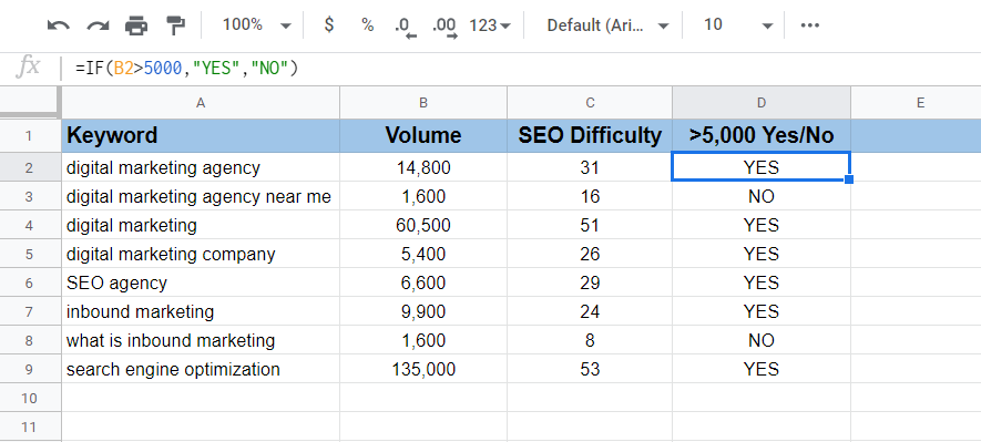
Once I enter the formula for the first keyword and press enter, I can drag from the first cell (D2) down the column, and the answers will auto-fill.
All the keywords with traffic over 5,000 visitors per month show up as “YES,” and those with traffic under 5,000 show up as “NO.”
You can also use the following functions with this equation:
3. Set a Default for Errors with IFERROR
Let’s say one of your cells shows an error message – which could show up as “#ERROR!” or “#DIV/0!” or “#VALUE!” – when you try to run a formula.
Error prompts can happen if you divide by zero, or an unknown range is used. This can become a problem when you are trying to make calculations that involve these cells. It can also make your spreadsheet look messy and may be confusing when you present it to others.
IFERROR helps you sidestep this issue by replacing error values with default values that you set yourself.
Simply insert your original formula along with whatever you want your default value to be. You can even leave it blank and just type ” ” for value_if_error.
=IFERROR (original_formula, value_if_error)
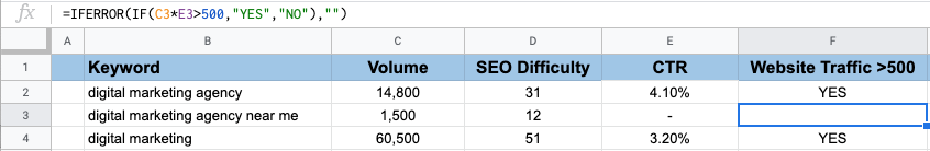
In this example, I want to find out which keywords could bring over 500 visitors to my website by multiplying search volume by click-through rate (CTR). Since “digital marketing agency near me” is (hypothetically) missing a CTR, it returns an error message.

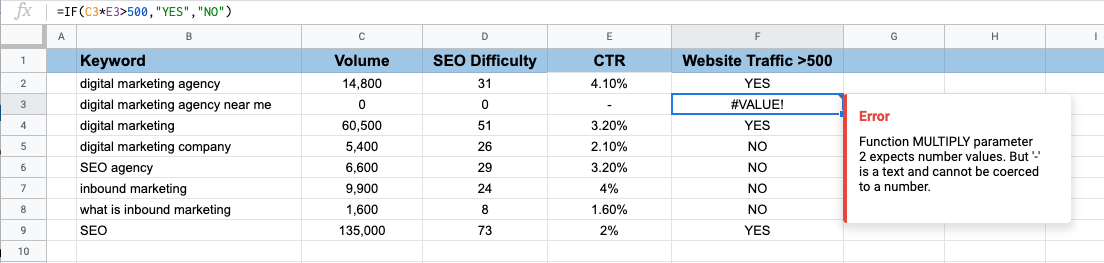
Instead of turning up an error message, I want this cell to remain blank, so I will wrap the equation in an IFERROR formula:
=IFERROR(IF(C3*E3>500,”YES”,”NO”),””)

4. SPLIT Your Data into Two Cells
Next up is the SPLIT formula:
=SPLIT(Text, Delimiter)
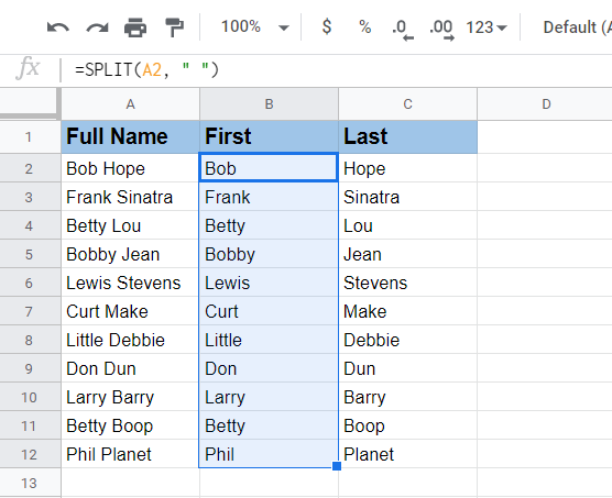
This allows you to split the data from one cell into multiple cells. Let’s say you have a spreadsheet of contacts with their full names in one column. To import your data correctly into your database, you need to split first and last names into two separate columns.
If I want to divide the names in column A into first and last names in columns B and C, my formula would be =SPLIT(A2, ” “) where A2 is the text I want to split up, and my delimiter is what separates the first and last names – a space in this case.
I’ll click on cell B2, and both B2 and C2 should populate once I enter the formula. Next is to drag from the first cell I populated (Bob) down to the last cell in the column (B12).
All first and last names will auto-populate for me.

5. Count Cells Quickly with COUNTIF
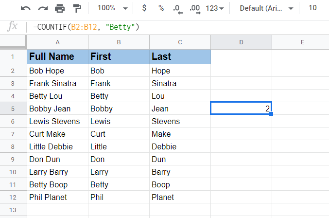
Say goodbye to counting cells manually. With the COUNTIF formula, you can count cells that meet specific criteria.
=COUNTIF(range, criteria)
This formula will not only save you time – but it’ll also make sure your numbers are accurate.
In my very simplified example below, I want to count all the cells in my spreadsheet that mention “Betty.” Here: =COUNTIF(B2:B15, “Betty”).
If I paste this formula into an empty cell, press “Enter,” and I will have my answer:

6. Apply One Formula to Multiple Cells with ARRAYFORMULA
You will love this one.
ARRAYFORMULA allows you to write out your formula one time and apply it to an entire row or column. You just take the formula you want to use and wrap it in an ARRAYFORMULA:
=ARRAYFORMULA(array_formula)
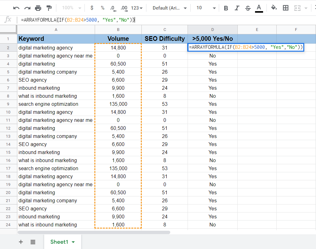
I have an IF formula I would like to use on column D below to determine which keywords get more than 5,000 visits each month. I select my first cell (D2) and paste my formula into the formula box.
I just need to be sure to include my first and last cells in my formula, i.e., B2 and B24. Then I press enter, and the column auto-populates.
=ARRAYFORMULA(IF(B2:B24>5000, “Yes”,”No”))

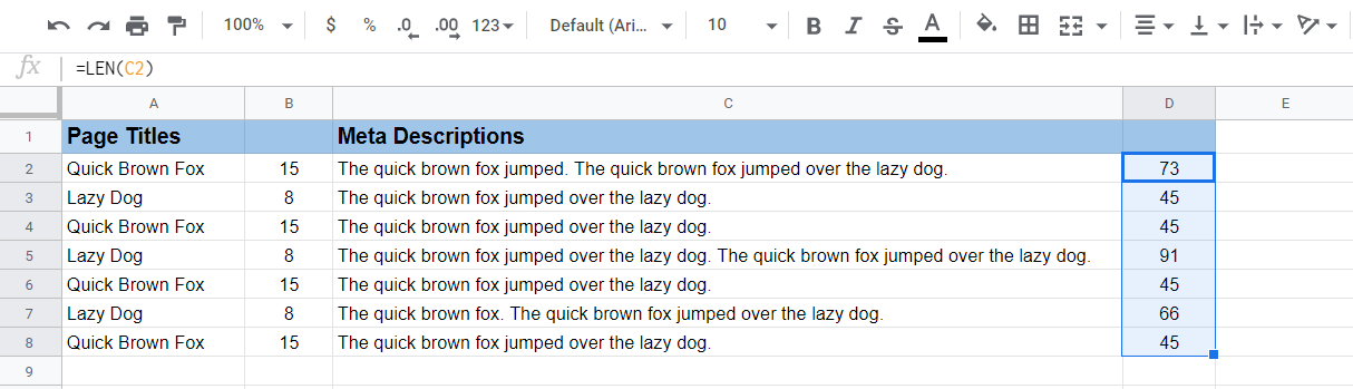
7. Use LEN to Count Characters
The LEN formula helps you count the number of characters in a cell.
=LEN(insertcell)
Let’s say you are reviewing meta descriptions and page titles for all your website pages in a spreadsheet, and you want to count the characters to make sure they are all the right length.
Click on a blank cell and enter the formula, replacing “insertcell” with the cell that contains the characters you would like to count.
In my example, A2 is the first cell I’d like to count, so my formula would simply be =LEN(A2). I press enter afterward, and the character count appears.
I can then use this formula for the rest of my column by dragging from the first cell down to the last cell.

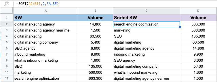
8. Easily SORT Your Cells
Want to sort your cells? You guessed it – we’ve got a formula for that. With the SORT formula, you can sort rows by the value in one or more columns. Use the formula =SORT(range, sort_column, is_ascending)
- Range is the group of cells you want to sort.
- Sort_column is the number (index) of the column you want to sort (A=1, B=2, etc.).
- If you want the values to sort in ascending order, simply mark “TRUE” for is_ascending. If you want values to sort in descending order, mark “FALSE” instead.
Let’s look at a simple example.
I want to see which of my top keywords have the highest search volume. Here is what my formula looks like:
=SORT(A2:B11,2,FALSE)

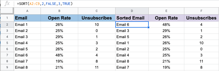
This formula comes in handy when you want to sort values in multiple columns. In the next example, I want to determine my top-performing emails.
I need to set up my formula, so the emails with the highest open rates and lowest unsubscribes appear first. My formula for this is =SORT(A2:C9,2,FALSE,3,TRUE)

9. Import Other Data with IMPORTRANGE
IMPORTRANGE is similar to VLOOKUP in that it allows you to import data from another Google Sheets spreadsheet.
=IMPORTRANGE(spreadsheet_url, range_string)
- Replace spreadsheet_url with the URL of the other spreadsheet, and then specify the range of cells you would like to import.
If you have multiple tabs in the spreadsheet you want to pull from, you will need to specify.
Let’s say you are pulling from a tab called “Keywords,” and you want the data from cells A2 to H150. Your formula would look like this:
=IMPORTRANGE(“https://docs.google.com/spreadsheets/d/1wID3VSaNi1zbiaQPZ”, “Keywords!A1:H150”)
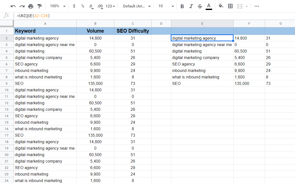
10. Keep Only The UNIQUE Data
Those of us who work with a lot of data know full well how often duplicate information can show up. The UNIQUE formula can help here.
Sometimes, you need to merge multiple family members into a single household, or one person ends up in your system twice by signing up for your newsletter multiple times under different email addresses.
There is a myriad of ways data can be duplicated, but this problem can quickly turn our spreadsheets and content management systems into huge sloppy messes. That is where this formula can help.
=UNIQUE(range)
In this example, I clicked on an empty cell and entered the formula =UNIQUE(A2:C24) to include all three columns of data; then I hit enter.
Voila!
All duplicate fields are removed, and the unique fields remain.

11. SEARCH for a Specific Value
The SEARCH formula can be used to check a set of data for a certain value.
For instance, let’s say you have all the URLs from your website listed in a spreadsheet and want to identify all of your blog articles.
Instead of going through and manually picking out all the blog posts, you can use this formula:
=SEARCH(search_query, text_to_search)
To flag all your blog posts as “Blog,” you’ll need to combine the above formula with the IF formula, which we covered above.
Here is what it could look like: =IF(SEARCH(“/blog/”,A2),”Blog”,””)
The formula will pull out all URLs containing /blog/ starting with cell A2.
URLs that don’t contain /blog/ will pull up an error message (#VALUE!). To avoid this, you can wrap this formula in an IFERROR formula to label non-blog URLs as “Other” (or leave it blank) and keep your data clean and error-free.
=IFERROR (IF(SEARCH(“/blog/”,A2),”Blog”,””), “Other”)
12. Add Dates Using TODAY
Entering dates into Google Sheets spreadsheets doesn’t have to be a pain anymore. This formula will help you fill out date ranges for reports faster than you have ever done before.
If you want to add today’s date, all you need to do is add the following formula to your cell:
=TODAY()
You don’t even need to know the date; it will automatically grab it for you.
If you want to figure out a date two or three weeks back without having to pull up a calendar, just add to your formula the number of days back you want to go.
=TODAY() – 14
This will show you the date exactly 14 days ago.
Conversely, if you want to grab a date in the future, simply add the number of days instead of subtracting.
=TODAY() + 7
In the above case, you’d see the date 7 days from today.
Pretty nifty, right?
13. Merge Cell Data with CONCATENATE
We have already learned how to split data into cells, but what about merging cell data? This formula is useful for working with URLs.
Sometimes, when you download a list of URLs, the website addresses aren’t formatted the way you want them.
Maybe you downloaded a list from Google Analytics, and the domain is missing. Or maybe the URLs are missing the leading protocol.
Instead of manually updating each URL individually, you can use the CONCATENATE formula.
=CONCATENATE(range)
Once you do the first one, simply pull down from the first box where you entered the formula, and the remaining cells will automatically populate.

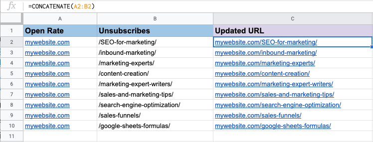
If a single prefix or suffix is not present in the sheet, you could manually insert it also without needing to create an extra column of cells for it – where the formula would look like =CONCATENATE(“https://”,A2)
14. Find Category Totals With SUMIF
The SUMIF formula can be useful for adding categories of values based on a specific criterion.
=SUMIF(range, criterion, [sum_range])
In the example below, I want to add up the page views of my top-performing blog posts to determine which blog category is the most popular. I can quickly add up page views by applying this formula for each category.
To calculate the page views in the SEO category:
- The range includes the column of cells under “Category”.
- “SEO” is the criterion.
- The sum_range includes the cells in the column under “Page Views”.
The formula will add up the number of total page views in the SEO category: 36,834. I will use this same formula for the other three categories and just switch the criterion for each.

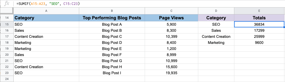
Without having to sort or make any extra calculation, I am able to observe the totals for each blog category and easily determine which category of blog post gets the most page views.
Keep These Powerful Formulas On Hand
Now you know some helpful formulas and functions to use in Google Sheets to make your spreadsheet life SO MUCH EASIER as a professional SEO.
Bookmark this page to keep these formulas handy, so you can quickly copy and paste them as you are working. We hope they can help you report, organize, and present data much more quickly and professionally (and let you show off your new skills a little in the process)!